Loss Development Modeling
This tutorial walks through a typical loss development workflow using LedgerAnalytics.
from ledger_analytics import AnalyticsClient

# If you've set the LEDGER_ANALYTICS_API_KEY environment variable
client = AnalyticsClient()

# alternatively
api_key = "..."
client = AnalyticsClient(api_key)
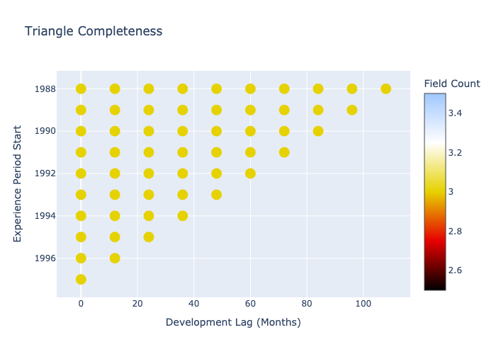
The Bermuda library comes equipped with a sample triangle containing paid loss, reported loss and earned premium. It’s a 10x10 annual triangle, so we’ll clip off the lower-right leaving a typical triangle-shaped loss development triangle, and load it into the API. We can also use Bermuda to plot the ‘data completeness’ of this triangle, providing a high-level view of it’s structure.
from datetime import date
from bermuda import meyers_tri

clipped_meyers = meyers_tri.clip(max_eval=date(1997, 12, 31))
dev_triangle = client.triangle.create(name="clipped_meyers_triangle", data=clipped_meyers)
clipped_meyers.plot_data_completeness()
Let’s see which models are available to us for loss and tail development.
client.development_model.list_model_types()
client.tail_model.list_model_types()
We’ll start with body development models. We’ll use the standard ChainLadder
development model for now, but the data get’s stale and thin after the
first few years, so we’ll switch to a tail model after a development
lag of 84 months. We expect that new loss development is more predictive
of future loss development patterns, so we can add exponential recency decay
based on the evaluation date.
chain_ladder = client.development_model.create(
    triangle=dev_triangle,
    name="paid_body_development",
    model_type="ChainLadder",
    config={
        "loss_definition": "paid",
        "recency_decay": 0.8
    }
)
Now we’ll need to fit a tail model to account for lags after 72 months. For this we’ll
use a GeneralizedBondy model which is a generalization of the classic Bondy model.
bondy = client.tail_model.create(
    triangle=dev_triangle,
    name="paid_bondy",
    model_type="GeneralizedBondy",
    config={
        "loss_definition": "paid",
    }
)
Now we can square this triangle using a combination of body development via the chain_ladder model and
tail development using Generalized Bondy. Note that by default the prediction triangle will be named "paid_body_clipped_meyers_triangle" based on the model_name and the triangle name. You have the option of passing in a different prediction_name to the predict method that will save the output triangle with a user-specified name.
chain_ladder_predictions = chain_ladder.predict(
    triangle=dev_triangle,
    config={"max_dev_lag": 84},
)

(clipped_meyers + chain_ladder_predictions.to_bermuda()).plot_data_completeness()
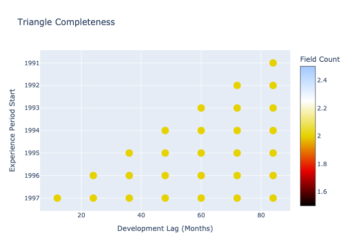
From the data completeness plot you can see the predictions out to dev lag 84 months, which are colored differently to the original data in green due to the different number of fields. Now we can apply the bondy model to a combination of these predcitions and the original triangle.
tail_pred_triangle = clipped_meyers + chain_ladder_predictions.to_bermuda()
client.triangle.create(name="tail_pred_triangle", data=tail_pred_triangle)
bondy_predictions = bondy.predict(
triangle="tail_pred_triangle",
config={"max_dev_lag": 120}
)
squared_triangle = tail_pred_triangle + bondy_predictions.to_bermuda()
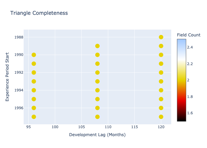
squared_triangle.plot_data_completeness()
The tail model predictions take us from lag 84 to lag 120.
For each future cell in the triangle there is a posterior distribution off 10,000 samples of paid losses.These distributions can be fed directly into a forecast model to predict the ultimate loss ratios for a future accident year. Reserves can be set using a selected quantile from these ultimate loss distributions.
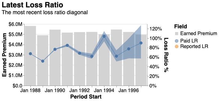
We can use Bermuda’s plotting tools to help us explore these predictions. For example, here’s the triangle’s ‘right edge’ after applying our loss development models.
squared_triangle.plot_right_edge()
The uncertainty intervals reflect that there is more uncertainty about the future loss ratios for the greener accident years, as we’d expect.
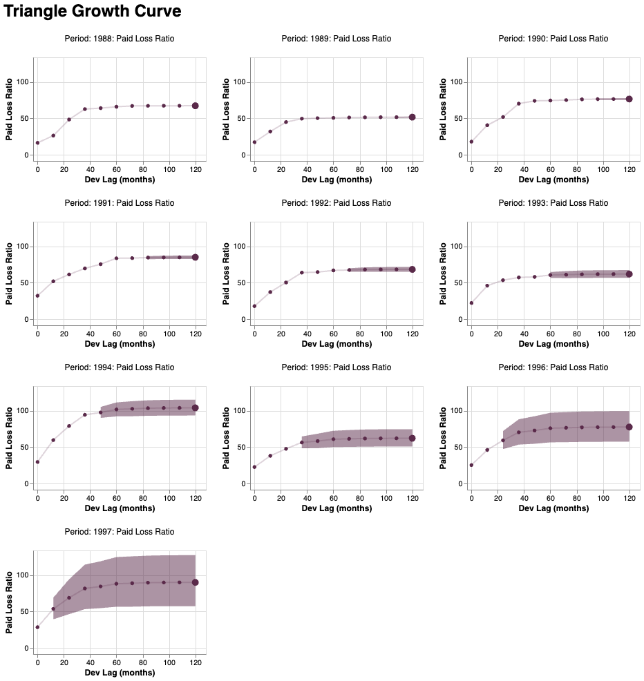
We can also look at the predictions for each accident year separately using more complex Bermuda plotting code, which uses Altair on the backend.
squared_triangle.derive_metadata(
    period = lambda cell: cell.period_start.year
).plot_growth_curve(
    width=250,
    height=150,
    ncols=3,
).resolve_scale(
    y="shared",
    x="shared",
    color="independent",
)
Check out the Bermuda library for more plotting options.